
The purpose of this article is to explore the basic principles regarding how an antenna radiates.
Some explanations of electromagnetic phenomena have been around for many years [1] but very little has found its way into amateur radio literature. It is hoped that the following will help to clear up the some of the mysteries of 'near' and 'far' fields and the differences between radiation resistance and ohmic resistance in an antenna.
The final part of the article describes how electromagnetic waves were discovered.
Sources used are indicated by a number in square brackets and referenced at the end.
Conductors and Insulators.
As you are all probably all aware, the atomic structure of material is most often described as being planetary in nature, a model first proposed in 1913 by Niels Bohr. In this model electrons orbit a nucleus as planets orbit a star in a solar system. The electron's orbital velocity and mass are in balance with the electrical force between the electron (arbitrary assigned negative) and the nucleus (positive). In a copper atom 29 electrons orbit the nucleus at four specific distances known as shells. The electron in the outer shell is easily detached from the atom by any weak field; these electrons are termed free electrons. At room temperature there are trillions of free electrons moving randomly from atom to atom. When an external electrical force, such as voltage from a battery, is applied to the conductor then the free electrons migrate from atom to atom.
Unlike copper most materials, say, wood, are not good conductors; they are instead insulators or ‘dielectrics’. In them, comparatively few electrons are available to move in response to the impressed electric or magnetic field. Of course there’s some movement or ‘displacement’ of electrons, the stronger the electric field, the greater the displacement.
Fundamental Stuff [2]
The difficulty about really fundamental things like electric charges is that there is nothing more fundamental that can be used to describe them. When I described an atom of copper above, electrons were mentioned. Now although we can say a lot about what the electrons do we cannot say what they are. So fundamental things can only be discussed in terms of mental pictures, like the Bohr model of the atom. We also use analogies and mathematical concepts, etc., such as 'lines of force'. This is very helpful in enabling people make practical use of things they really don’t understand. The fact that nobody knows what electrons are has not prevented them being used in most complicated and ingenious ways.
Usually all concerned manage to agree to use the same mental pictures when they discuss these fundamental things or perform the calculations necessary to exploit them to the best advantage.
Although these concepts are so helpful, and it is difficult to see how we could carry on engineering and other applied sciences without them, they are dangerously liable to mislead us into accepting them as realities.
Take 'lines of force' for example. We know by experiment that exceptional things happen in the space around what we are pleased to call 'electrically charged bodies'. We just don’t understand why or how these things happen, but it has been found by careful study that they always happen in certain definite ways and with certain numerical relationships. So scientists have defined various quantities such as charge and potential, and have enunciated various laws connecting them, and to help you and me to grasp these they have imagined; such things as 'lines of force'. Owing to the care with which these things have been defined, they make up a consistent system, and one can work about with them and design electrical and radio appliances and predict their performance with confidence. But they are quite arbitrary. If aliens in a planet in the outer fringes of Andromedia are using radio technology they will no doubt have developed completely different ways of thinking about the subject.
The Electron and the E-Field [1] [3]
The electric force of an electron has already been mentioned. The electron is visualised in Fig 1A as a spherical object, which is the source of an electric field known as the E-Field. This field diverges from the electron; that is, it spreads out in three dimensions from that electron in straight lines until it reaches the limits of the universe. In reality most of the E lines from an electron will not go to infinity, but will rather go toward some positive charge, say a hydrogen nucleus (proton) nearby. Initially we will simplify our model by considering a universe that consists of one individual electron..

Fig 1: A. Diverging lines of force from an electron. This is a two-dimensional picture; the lines of force from an electron radiated in three dimensions. B. If the electron is suddenly moved a discontinuity in these lines of force will occur. This discontinuity moves away from the electron at the speed of light.
If the electron is suddenly moved to a different position there will also be a shift in the lines of force. This causes kinks in these lines, see Fig 1B, which move away from the electron at the speed of light.
To simplify the visualisation process we will now only consider one E line associated with this electron. As shown in Fig 2A, a sudden shift in the position of our electron has produce a 'kink' in the E field line, which is travelling away from the electron.

Fig 2. (A) A kink in an E-field line due to the movement of the electron which produced the field. (B) Continuously wiggled electron (up and down) creates a continuously radiating e-field. (C) An H field created by the E-field. (D) An electromagnetic wave, comprising E and H fields with their phases in locked together and their vectors at a right angles to each other.
This kink propagates away from the electron, updating the rest of the field that has lagged behind Part of the energy exerted by the force that moved the electron is expended to propagate the kink in the field. Therefore, the kink carries with it radiating energy; and because the field diverges in all directions, as shown in Fig 1 the energy radiates in all directions.
The strength of the kink depends on how quickly the electron is moved from one position to the next (acceleration). To make the field radiate continuously the electron must be continuously wiggled or vibrated, see Fig 2(B).
The Magnetic Field [1] [3]
We all know that there is a magnetic field associated with any movement of electrons (current flow) and if the current varies so does the magnetic field. Thus our oscillating electron creates an oscillating magnetic field, known as the H-Field as shown in Fig 2(C).
In the same instant that we are producing a vertically oriented E field, (using the orientation shown in Fig 2(B), we are also producing a horizontally oriented H field. These two fields will be in time phase; that is, the peak of the sine wave will be the same in the E and the H fields, see Fig 2(D). These two fields are locked together due to the fact that they were produced by a single event, the acceleration of the electron. They will always travel along with their phases in locked together and their vectors at a right angle to each other. Such a wave is called an Electromagnetic (EM) wave
The Big Picture [3] [4]
A single electron won't produce a very powerful EM wave, no matter how fast or how much it is vibrated, so practical antennas vibrate lots of electrons at some rather high accelerations.
We know that an electric current in a conductor is simply a mass migration of free electrons. If the current is alternating, as in an antenna, the free electrons in a given locality vibrate back and forth in unison driven by a potential supplied by the transmitter. Evidently, then, any individual electron moves to and fro around an average position. Let's see how far and how fast this electron might travel.
Consider an antenna made of 2.5mm diameter copper wire and being excited by a transmitter on 14.1 MHz. Each free electron near the surface of the wire is executing 14.1 million cycles of motion per second. Knowing the number of free electrons per cubic mm of copper, the electric charge on each, and the depth of RF penetration into the wire (the skin depth), we can calculate the peak speed of an electron at a place where the RMS antenna current is, say, one ampere. The result comes out to be less than 10mm per second. At that rate the electron doesn't move very far during each half cycle of vibration, its peak-to-peak travel being less than a millionth of a millimeter. From an electron's perspective this distance is quite respectable, being tens of thousands of times its own diameter.
We can compute the electron's deceleration and acceleration, which are greatest when the electron is coming to a stop and then starting up in the other direction. At an antenna current of one ampere, these quantities reach more than 50.000 gs.
A hot lamp filament is also decelerating and accelerating a lot of electrons, but they are in random phase. Therefore, the contributions of the individual electrons add at random. We call this 'incoherent' light. A laser and an antenna decelerate and accelerate all of the electrons in phase so that a distant EM waves all add in phase.
A Digression - The Nature of Space [3]
Empty space is a medium through which energy can be transmitted. It has zero gain and no attenuation. Furthermore, it is perfectly linear, which means that the weakest signals and the most powerful can be accommodated without interaction. For example, the tiny signals from the most distant space probe can be received in the presence of all the broadcast transmissions on the planet and the colossal level of EM energy from the sun. Because these fields do not interact then we can assume that the vector sum of a number of fields will be the simple sum and not include some product terms as would be the case if space were non-linear. This is known as the principle of superposition.
One of the implications of superposition is that we can consider each electron individually when it comes to the generation of EM waves. Then, we can simply add up the effects of each electron to determine the overall strength of EM waves in all space. Fortunately, superposition teaches us that we can also do our analysis by taking a group of electrons here and another there and once the effects of each group has been determined, we can add them all together to get the total effect.
The speed at which the energy spreads is determined by the characteristics of space. These characteristics include both a non-zero dielectric constant (permittivity Note 1), which permits space to store energy in an E field, and a non-zero magnetic constant (permeability Note 2) which permits space to store energy in an H field. These combine to produce a definite value for C, the speed of propagation of EM waves in space, better known as the speed of light.
Its electric permittivity and magnetic permeability determine its characteristic impedance, which is about 377 ohms
Near Fields [3]
In the real world of antennas our ability to produce the ideal current configurations described above is limited. There are certain side effects; one of these is the production of so called 'near' fields.
If we consider the dipole; once current begins flowing, charge will build up on the ends, simply because it has nowhere to go. This charge will produce a voltage between one end of the dipole and the other and will thus be, in effect, be a capacitor. There will be E fields from the positive pole of the capacitor to the negative pole. These E fields, being part of a capacitor, are reactive or 'near' fields.
The H fields produced by the current in a dipole are directly the result of RF currents and are therefore part of the radiated wave. However, in a dipole there will be near H fields produced by the displacement currents, which exist while the E field is building or collapsing. These near E and near H fields, unlike the EM waves produced by oscillating electrons, are not coupled. Their ratios can be individually controlled, for example, by changing the geometry of the dipole. Furthermore, the H field reaches its maximum when the E field is changing the fastest, and the capacitive E field its maximum when the voltage at the ends of the dipole are maximum. Therefore, the two fields in Fig 3 are not in time phase, like the E and H in the EM wave shown in Fig 2D. This is why the near fields do not radiate, but simply store energy in the immediate vicinity of the antenna. We would just as soon do without them, but they are an inevitable 'parasitic' effect of the operation of the antenna.

Fig 3: The E and H fields are produced individually by either a current or a voltage and do not affect each other in any way. These E and H fields exist in relatively close proximity to the antenna, are 180 degrees out of phase with each other and, collectively known as the reactive or near field.
Near field strengths die out very quickly with distance from the antenna. Thus, when measuring the gain or pattern of an antenna, one must be sure to be in the region where the near fields have fallen well below the radiated fields or a false result will be obtained. This danger has led some to draw false conclusions in the past about a particular antenna's performance. We could avoid this source of error if instruments could be made that only measured EM waves and did not respond to reactive E or H fields.
Radiation Resistance Versus Ohmic Resistance [4]
The radiation and induction fields of a vibrating electron exist right down to the electron. Since the electron carries an electric charge, and since an electric charge is pulled by an electric field it follows that a force is exerted on the very electron that is producing them. The effect is a drag proportional to speed, as if the electron were moving through a viscous fluid. This drag force is the cause of radiation resistance.
An electron moving in a conductor also feels a drag force that is due to frequent progress-impeding collisions between the electron and the atoms in its path. This drag is the cause of ohmic resistance, the familiar R in Ohm's Law.
Both kinds of resistance dissipate energy at a rate equal to the resistance times the square of the current. Of course, energy dissipated this way doesn't actually disappear. An alternating current, flowing against radiation resistance, turns electrical energy into radiant energy, which wings its way off into space. Current flowing against ohmic resistance transforms electrical energy into heat, which is mechanical vibration of the atoms of the conductor - the atoms vibrate when they're hit by the moving free electrons.
Radiation resistance varies along the length of an antenna wire, but it is independent of the diameter and material of the conductor. The middle third of a half-wave. 14MHz dipole has a radiation resistance of 1.3 ohms per 100mm. That's nearly 80 times the ohmic resistance of clean 2.5mm copper wire at this frequency. Closer to the ends of the antenna, the radiation resistance is even higher.
How Radio Waves were Discovered [5]
Earlier, I mentioned the work of individuals who defined various quantities and enunciating various laws connecting them. Some of the most important of these are:
Charles Augustin de Coulomb (1736 - 1806). Devised mathematical formula used to calculate the force between two charged bodies (Coulomb's Law).
Count Alessandro Volta (1745 - 1827). Inventor of the battery and the capacitor.
Andre-Marie Ampere (1775 - 1836). Invented the electromagnet and defined the unit of current.
Michael Faraday (1791 -1867). Discovered and defined electromagnetic induction
In 1873, James Clerk Maxwell (1831 - 1879) published the first unified theory of electricity and magnetism based mainly on the experimental work of Faraday. This work led to him to postulate the existence of electromagnetic waves. A simplified, intelligible and non-mathematical explanation of how Maxwell discovered electromagnetic waves quoted below is by Paul Sagan [5].
"Here they are, the four Maxwell equations for the behaviour of electricity and magnetism in matter:
Ñ . E = r/e0
Ñ . B = 0
Ñ x E = -B!
Ñ x B = m0j + m0 e0E!
(Note: In the original B! is B with a dot above it and E! an E with a dot above it, beyond the capabilities of my system)
"It takes a few years of university-level physics to understand these equations. They are written using a branch of mathematics called vector calculus. A vector, written in bold-face type, is any quantity with both a magnitude and a direction. Sixty km an hour isn’t a vector, but sixty km an hour due north on the M1 motorway is.
"E and B represent the electric and magnetic fields. The triangle, called a nabla (because of its resemblance to a certain ancient Middle Eastern harp), expresses how the electric or magnetic fields vary in three-dimensional space. The ‘dot product’ and the ‘cross product’ after the nablas are statements of two different kinds of spatial variation.
E! and B! represent the time variation, the rate of change of the electric and magnetic fields. j stands for the electrical current. The lower-case Greek letter r (rho) represents the density of electrical charges, while e0 (epsilon zero) and m0 (mu zero) are not variables, but properties of the substance E and B are measured in, and determined by experiment. In a vacuum, e0 and m0 are constants of nature (see notes 1 and 2).
Considering how many different quantities are being brought together in these equations. it’s striking how simple they are. They could have gone on for pages, but they don’t.
The first of the four Maxwell equations tells how an electric field due to electrical charges (electrons, for example) varies with distance (it gets weaker the farther away we go). But the greater the charge density (the more electrons, say. in a given space) the stronger the field.
The second equation tells us that there’s no comparable statement in magnetism, because magnetic ‘charges’ (or magnetic ‘monopoles’) do not exist: Saw a magnet in half and you won’t be holding an isolated 'north' pole and an isolated 'south' pole; each piece now has its own ‘north’ and ‘south’ pole. The third equation tells us how a changing magnetic field induces an electric field. The fourth describes the converse - how a changing electric field (or an electrical current) induces a magnetic field
"The four equations are essentially distillations of generations of laboratory experiments performed by the individuals (and others) named above. What is described here vaguely and qualitatively, the equations describe exactly and quantitatively.
Maxwell then asked himself a strange question: what would these equations look like in empty space, in a vacuum, in a place where there were no electrical charges and no electrical currents? We might very well anticipate no electric and no magnetic fields in a vacuum. Instead, he suggested that the right form of the Maxwell equations for the behaviour of electricity and magnetism in empty space is this:
Ñ . E = 0
Ñ . B = 0
Ñ x E = -B!
Ñ x B = m0 e0E!
"He set r equal to zero, indicating that there are no electrical charges. He also set j equal to zero, indicating that there are no electrical currents. But he didn’t discard the last term in the fourth equation, m0 e0E!, the feeble displacement current in insulators.
"Why not? As you can see from the equations, Maxwell’s intuition preserved the symmetry between the magnetic and electric fields. Even in a vacuum, in the total absence of electricity, or even matter, a changing magnetic field, he proposed, elicits an electric field and vice versa. The equations were to represent the elegance of Nature. (There was also another, more technical reason for preserving the displacement current in a vacuum, which is beyond the scope of this article.)
"Briefly, the four Maxwell equations for a vacuum say (1) there are no electrical charges in a vacuum; (2) there are no magnetic monopoles in a vacuum; (3) a changing magnetic field generates an electrical field; and (4) vice versa.
When all the equations were written down like this, Maxwell was readily able to show that E and B propagated through empty space as if they were waves. What’s more, he could calculate the speed of the wave. It was just 1 divided by the square root of e0 times m0. But e0 and m0 had been measured in the laboratory. When the numbers where plugged in it was found that the electric and magnetic fields in a vacuum appeared to propagate, astonishingly, at the same speed as had already been measured for light, see Note [3]. The agreement was too close to be accidental. Suddenly, disconcertingly, electricity and magnetism were deeply implicated in the nature of light. Since light now appeared to behave as waves and to derive from electric and magnetic fields Maxwell called it electromagnetic."
And Finally
The professional radio engineer and mathematical purist will probably deem this article simplistic and rightly so. However, there can be many different levels of understanding on any subject, and we must recognise that at all these levels, all we have are models at different levels of sophistication. Furthermore, a simple model may help us sort out the wood from the trees. It is not unusual to see scientific papers, which are so obscure that we have to rely on the supposed veracity of the authors, or on the logical soundness of the mathematics. More than once in the past has an unsound antenna design been be hidden beneath logically correct and incorrect mathematics.
Some explanations of electromagnetic phenomena have been around for many years [1] but very little has found its way into amateur radio literature. It is hoped that the following will help to clear up the some of the mysteries of 'near' and 'far' fields and the differences between radiation resistance and ohmic resistance in an antenna.
The final part of the article describes how electromagnetic waves were discovered.
Sources used are indicated by a number in square brackets and referenced at the end.
Conductors and Insulators.
As you are all probably all aware, the atomic structure of material is most often described as being planetary in nature, a model first proposed in 1913 by Niels Bohr. In this model electrons orbit a nucleus as planets orbit a star in a solar system. The electron's orbital velocity and mass are in balance with the electrical force between the electron (arbitrary assigned negative) and the nucleus (positive). In a copper atom 29 electrons orbit the nucleus at four specific distances known as shells. The electron in the outer shell is easily detached from the atom by any weak field; these electrons are termed free electrons. At room temperature there are trillions of free electrons moving randomly from atom to atom. When an external electrical force, such as voltage from a battery, is applied to the conductor then the free electrons migrate from atom to atom.
Unlike copper most materials, say, wood, are not good conductors; they are instead insulators or ‘dielectrics’. In them, comparatively few electrons are available to move in response to the impressed electric or magnetic field. Of course there’s some movement or ‘displacement’ of electrons, the stronger the electric field, the greater the displacement.
Fundamental Stuff [2]
The difficulty about really fundamental things like electric charges is that there is nothing more fundamental that can be used to describe them. When I described an atom of copper above, electrons were mentioned. Now although we can say a lot about what the electrons do we cannot say what they are. So fundamental things can only be discussed in terms of mental pictures, like the Bohr model of the atom. We also use analogies and mathematical concepts, etc., such as 'lines of force'. This is very helpful in enabling people make practical use of things they really don’t understand. The fact that nobody knows what electrons are has not prevented them being used in most complicated and ingenious ways.
Usually all concerned manage to agree to use the same mental pictures when they discuss these fundamental things or perform the calculations necessary to exploit them to the best advantage.
Although these concepts are so helpful, and it is difficult to see how we could carry on engineering and other applied sciences without them, they are dangerously liable to mislead us into accepting them as realities.
Take 'lines of force' for example. We know by experiment that exceptional things happen in the space around what we are pleased to call 'electrically charged bodies'. We just don’t understand why or how these things happen, but it has been found by careful study that they always happen in certain definite ways and with certain numerical relationships. So scientists have defined various quantities such as charge and potential, and have enunciated various laws connecting them, and to help you and me to grasp these they have imagined; such things as 'lines of force'. Owing to the care with which these things have been defined, they make up a consistent system, and one can work about with them and design electrical and radio appliances and predict their performance with confidence. But they are quite arbitrary. If aliens in a planet in the outer fringes of Andromedia are using radio technology they will no doubt have developed completely different ways of thinking about the subject.
The Electron and the E-Field [1] [3]
The electric force of an electron has already been mentioned. The electron is visualised in Fig 1A as a spherical object, which is the source of an electric field known as the E-Field. This field diverges from the electron; that is, it spreads out in three dimensions from that electron in straight lines until it reaches the limits of the universe. In reality most of the E lines from an electron will not go to infinity, but will rather go toward some positive charge, say a hydrogen nucleus (proton) nearby. Initially we will simplify our model by considering a universe that consists of one individual electron..
Fig 1: A. Diverging lines of force from an electron. This is a two-dimensional picture; the lines of force from an electron radiated in three dimensions. B. If the electron is suddenly moved a discontinuity in these lines of force will occur. This discontinuity moves away from the electron at the speed of light.
If the electron is suddenly moved to a different position there will also be a shift in the lines of force. This causes kinks in these lines, see Fig 1B, which move away from the electron at the speed of light.
To simplify the visualisation process we will now only consider one E line associated with this electron. As shown in Fig 2A, a sudden shift in the position of our electron has produce a 'kink' in the E field line, which is travelling away from the electron.
Fig 2. (A) A kink in an E-field line due to the movement of the electron which produced the field. (B) Continuously wiggled electron (up and down) creates a continuously radiating e-field. (C) An H field created by the E-field. (D) An electromagnetic wave, comprising E and H fields with their phases in locked together and their vectors at a right angles to each other.
This kink propagates away from the electron, updating the rest of the field that has lagged behind Part of the energy exerted by the force that moved the electron is expended to propagate the kink in the field. Therefore, the kink carries with it radiating energy; and because the field diverges in all directions, as shown in Fig 1 the energy radiates in all directions.
The strength of the kink depends on how quickly the electron is moved from one position to the next (acceleration). To make the field radiate continuously the electron must be continuously wiggled or vibrated, see Fig 2(B).
The Magnetic Field [1] [3]
We all know that there is a magnetic field associated with any movement of electrons (current flow) and if the current varies so does the magnetic field. Thus our oscillating electron creates an oscillating magnetic field, known as the H-Field as shown in Fig 2(C).
In the same instant that we are producing a vertically oriented E field, (using the orientation shown in Fig 2(B), we are also producing a horizontally oriented H field. These two fields will be in time phase; that is, the peak of the sine wave will be the same in the E and the H fields, see Fig 2(D). These two fields are locked together due to the fact that they were produced by a single event, the acceleration of the electron. They will always travel along with their phases in locked together and their vectors at a right angle to each other. Such a wave is called an Electromagnetic (EM) wave
The Big Picture [3] [4]
A single electron won't produce a very powerful EM wave, no matter how fast or how much it is vibrated, so practical antennas vibrate lots of electrons at some rather high accelerations.
We know that an electric current in a conductor is simply a mass migration of free electrons. If the current is alternating, as in an antenna, the free electrons in a given locality vibrate back and forth in unison driven by a potential supplied by the transmitter. Evidently, then, any individual electron moves to and fro around an average position. Let's see how far and how fast this electron might travel.
Consider an antenna made of 2.5mm diameter copper wire and being excited by a transmitter on 14.1 MHz. Each free electron near the surface of the wire is executing 14.1 million cycles of motion per second. Knowing the number of free electrons per cubic mm of copper, the electric charge on each, and the depth of RF penetration into the wire (the skin depth), we can calculate the peak speed of an electron at a place where the RMS antenna current is, say, one ampere. The result comes out to be less than 10mm per second. At that rate the electron doesn't move very far during each half cycle of vibration, its peak-to-peak travel being less than a millionth of a millimeter. From an electron's perspective this distance is quite respectable, being tens of thousands of times its own diameter.
We can compute the electron's deceleration and acceleration, which are greatest when the electron is coming to a stop and then starting up in the other direction. At an antenna current of one ampere, these quantities reach more than 50.000 gs.
A hot lamp filament is also decelerating and accelerating a lot of electrons, but they are in random phase. Therefore, the contributions of the individual electrons add at random. We call this 'incoherent' light. A laser and an antenna decelerate and accelerate all of the electrons in phase so that a distant EM waves all add in phase.
A Digression - The Nature of Space [3]
Empty space is a medium through which energy can be transmitted. It has zero gain and no attenuation. Furthermore, it is perfectly linear, which means that the weakest signals and the most powerful can be accommodated without interaction. For example, the tiny signals from the most distant space probe can be received in the presence of all the broadcast transmissions on the planet and the colossal level of EM energy from the sun. Because these fields do not interact then we can assume that the vector sum of a number of fields will be the simple sum and not include some product terms as would be the case if space were non-linear. This is known as the principle of superposition.
One of the implications of superposition is that we can consider each electron individually when it comes to the generation of EM waves. Then, we can simply add up the effects of each electron to determine the overall strength of EM waves in all space. Fortunately, superposition teaches us that we can also do our analysis by taking a group of electrons here and another there and once the effects of each group has been determined, we can add them all together to get the total effect.
The speed at which the energy spreads is determined by the characteristics of space. These characteristics include both a non-zero dielectric constant (permittivity Note 1), which permits space to store energy in an E field, and a non-zero magnetic constant (permeability Note 2) which permits space to store energy in an H field. These combine to produce a definite value for C, the speed of propagation of EM waves in space, better known as the speed of light.
Its electric permittivity and magnetic permeability determine its characteristic impedance, which is about 377 ohms
Near Fields [3]
In the real world of antennas our ability to produce the ideal current configurations described above is limited. There are certain side effects; one of these is the production of so called 'near' fields.
If we consider the dipole; once current begins flowing, charge will build up on the ends, simply because it has nowhere to go. This charge will produce a voltage between one end of the dipole and the other and will thus be, in effect, be a capacitor. There will be E fields from the positive pole of the capacitor to the negative pole. These E fields, being part of a capacitor, are reactive or 'near' fields.
The H fields produced by the current in a dipole are directly the result of RF currents and are therefore part of the radiated wave. However, in a dipole there will be near H fields produced by the displacement currents, which exist while the E field is building or collapsing. These near E and near H fields, unlike the EM waves produced by oscillating electrons, are not coupled. Their ratios can be individually controlled, for example, by changing the geometry of the dipole. Furthermore, the H field reaches its maximum when the E field is changing the fastest, and the capacitive E field its maximum when the voltage at the ends of the dipole are maximum. Therefore, the two fields in Fig 3 are not in time phase, like the E and H in the EM wave shown in Fig 2D. This is why the near fields do not radiate, but simply store energy in the immediate vicinity of the antenna. We would just as soon do without them, but they are an inevitable 'parasitic' effect of the operation of the antenna.
Fig 3: The E and H fields are produced individually by either a current or a voltage and do not affect each other in any way. These E and H fields exist in relatively close proximity to the antenna, are 180 degrees out of phase with each other and, collectively known as the reactive or near field.
Near field strengths die out very quickly with distance from the antenna. Thus, when measuring the gain or pattern of an antenna, one must be sure to be in the region where the near fields have fallen well below the radiated fields or a false result will be obtained. This danger has led some to draw false conclusions in the past about a particular antenna's performance. We could avoid this source of error if instruments could be made that only measured EM waves and did not respond to reactive E or H fields.
Radiation Resistance Versus Ohmic Resistance [4]
The radiation and induction fields of a vibrating electron exist right down to the electron. Since the electron carries an electric charge, and since an electric charge is pulled by an electric field it follows that a force is exerted on the very electron that is producing them. The effect is a drag proportional to speed, as if the electron were moving through a viscous fluid. This drag force is the cause of radiation resistance.
An electron moving in a conductor also feels a drag force that is due to frequent progress-impeding collisions between the electron and the atoms in its path. This drag is the cause of ohmic resistance, the familiar R in Ohm's Law.
Both kinds of resistance dissipate energy at a rate equal to the resistance times the square of the current. Of course, energy dissipated this way doesn't actually disappear. An alternating current, flowing against radiation resistance, turns electrical energy into radiant energy, which wings its way off into space. Current flowing against ohmic resistance transforms electrical energy into heat, which is mechanical vibration of the atoms of the conductor - the atoms vibrate when they're hit by the moving free electrons.
Radiation resistance varies along the length of an antenna wire, but it is independent of the diameter and material of the conductor. The middle third of a half-wave. 14MHz dipole has a radiation resistance of 1.3 ohms per 100mm. That's nearly 80 times the ohmic resistance of clean 2.5mm copper wire at this frequency. Closer to the ends of the antenna, the radiation resistance is even higher.
How Radio Waves were Discovered [5]
Earlier, I mentioned the work of individuals who defined various quantities and enunciating various laws connecting them. Some of the most important of these are:
Charles Augustin de Coulomb (1736 - 1806). Devised mathematical formula used to calculate the force between two charged bodies (Coulomb's Law).
Count Alessandro Volta (1745 - 1827). Inventor of the battery and the capacitor.
Andre-Marie Ampere (1775 - 1836). Invented the electromagnet and defined the unit of current.
Michael Faraday (1791 -1867). Discovered and defined electromagnetic induction
In 1873, James Clerk Maxwell (1831 - 1879) published the first unified theory of electricity and magnetism based mainly on the experimental work of Faraday. This work led to him to postulate the existence of electromagnetic waves. A simplified, intelligible and non-mathematical explanation of how Maxwell discovered electromagnetic waves quoted below is by Paul Sagan [5].
"Here they are, the four Maxwell equations for the behaviour of electricity and magnetism in matter:
Ñ . E = r/e0
Ñ . B = 0
Ñ x E = -B!
Ñ x B = m0j + m0 e0E!
(Note: In the original B! is B with a dot above it and E! an E with a dot above it, beyond the capabilities of my system)
"It takes a few years of university-level physics to understand these equations. They are written using a branch of mathematics called vector calculus. A vector, written in bold-face type, is any quantity with both a magnitude and a direction. Sixty km an hour isn’t a vector, but sixty km an hour due north on the M1 motorway is.
"E and B represent the electric and magnetic fields. The triangle, called a nabla (because of its resemblance to a certain ancient Middle Eastern harp), expresses how the electric or magnetic fields vary in three-dimensional space. The ‘dot product’ and the ‘cross product’ after the nablas are statements of two different kinds of spatial variation.
E! and B! represent the time variation, the rate of change of the electric and magnetic fields. j stands for the electrical current. The lower-case Greek letter r (rho) represents the density of electrical charges, while e0 (epsilon zero) and m0 (mu zero) are not variables, but properties of the substance E and B are measured in, and determined by experiment. In a vacuum, e0 and m0 are constants of nature (see notes 1 and 2).
Considering how many different quantities are being brought together in these equations. it’s striking how simple they are. They could have gone on for pages, but they don’t.
The first of the four Maxwell equations tells how an electric field due to electrical charges (electrons, for example) varies with distance (it gets weaker the farther away we go). But the greater the charge density (the more electrons, say. in a given space) the stronger the field.
The second equation tells us that there’s no comparable statement in magnetism, because magnetic ‘charges’ (or magnetic ‘monopoles’) do not exist: Saw a magnet in half and you won’t be holding an isolated 'north' pole and an isolated 'south' pole; each piece now has its own ‘north’ and ‘south’ pole. The third equation tells us how a changing magnetic field induces an electric field. The fourth describes the converse - how a changing electric field (or an electrical current) induces a magnetic field
"The four equations are essentially distillations of generations of laboratory experiments performed by the individuals (and others) named above. What is described here vaguely and qualitatively, the equations describe exactly and quantitatively.
Maxwell then asked himself a strange question: what would these equations look like in empty space, in a vacuum, in a place where there were no electrical charges and no electrical currents? We might very well anticipate no electric and no magnetic fields in a vacuum. Instead, he suggested that the right form of the Maxwell equations for the behaviour of electricity and magnetism in empty space is this:
Ñ . E = 0
Ñ . B = 0
Ñ x E = -B!
Ñ x B = m0 e0E!
"He set r equal to zero, indicating that there are no electrical charges. He also set j equal to zero, indicating that there are no electrical currents. But he didn’t discard the last term in the fourth equation, m0 e0E!, the feeble displacement current in insulators.
"Why not? As you can see from the equations, Maxwell’s intuition preserved the symmetry between the magnetic and electric fields. Even in a vacuum, in the total absence of electricity, or even matter, a changing magnetic field, he proposed, elicits an electric field and vice versa. The equations were to represent the elegance of Nature. (There was also another, more technical reason for preserving the displacement current in a vacuum, which is beyond the scope of this article.)
"Briefly, the four Maxwell equations for a vacuum say (1) there are no electrical charges in a vacuum; (2) there are no magnetic monopoles in a vacuum; (3) a changing magnetic field generates an electrical field; and (4) vice versa.
When all the equations were written down like this, Maxwell was readily able to show that E and B propagated through empty space as if they were waves. What’s more, he could calculate the speed of the wave. It was just 1 divided by the square root of e0 times m0. But e0 and m0 had been measured in the laboratory. When the numbers where plugged in it was found that the electric and magnetic fields in a vacuum appeared to propagate, astonishingly, at the same speed as had already been measured for light, see Note [3]. The agreement was too close to be accidental. Suddenly, disconcertingly, electricity and magnetism were deeply implicated in the nature of light. Since light now appeared to behave as waves and to derive from electric and magnetic fields Maxwell called it electromagnetic."
And Finally
The professional radio engineer and mathematical purist will probably deem this article simplistic and rightly so. However, there can be many different levels of understanding on any subject, and we must recognise that at all these levels, all we have are models at different levels of sophistication. Furthermore, a simple model may help us sort out the wood from the trees. It is not unusual to see scientific papers, which are so obscure that we have to rely on the supposed veracity of the authors, or on the logical soundness of the mathematics. More than once in the past has an unsound antenna design been be hidden beneath logically correct and incorrect mathematics.




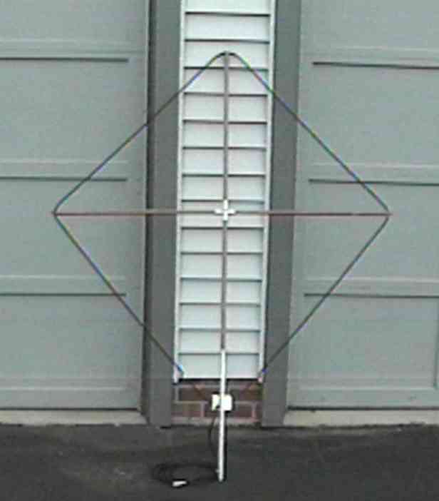


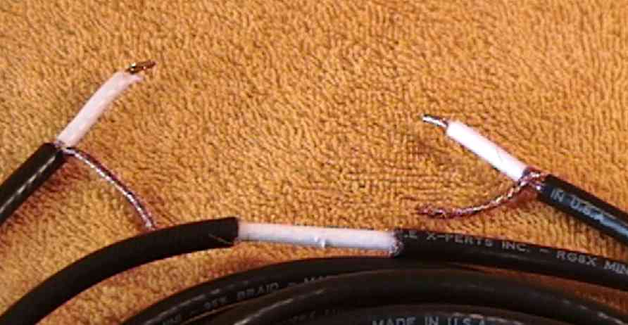
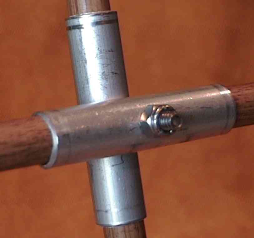


 To make this loop take 20 feet of RG59 coax. Half way along the coax , At the point that will become the top of the loop, break the shield for 1 inch. Place a variable trimmer capacitor (400pf) inside a waterproof project box. I mounted mine on some wood, with a hole drilled for the trimmer shaft to sit in. I glued the trimmer cap to the wood.

 I have also tried a 4.2m x 2.4m loop with excellent results on the LF bands. It seems to outperform the previous antenna on the LF bands by quite a large margin. The antenna is a corner fed loop as shown here.